Linear Regression

Linear Regression model is used to obtain relationship between a continuous outcome variable and one or more predictor variables. It is generally a good practice to understand the intution behind this approach. On the algorithm front, there are two techniques commonly used to optimize the parameters of the model, Normal Equation Method (uses Linear Algebra) and Gradient Descent (uses differential calculus, commonly used in a lot of Machine Learning Models).

Intution

General equation for linear regression with n independent variables is,

Y(x) = θ_o + θ₁x₁ + θ₂x₂ + … + θ_nx_n + ε

and the prediction equation is,

Ŷ(x) = h_θ(x) = θ_o + θ₁x₁ + θ₂x₂ + … + θ_nx_n

where, Y is actual dependent variable, x₁, x₂, …. , x_n are independent variables, h_θ(x) is predicted dependent variable, θ_o, θ₁, … , θ_n are coefficients of independent variables and ε is the error term.

The error metric considered here is Sum of Square of Error (SSE) because of which the model is also known as Ordinay Least Square (OLS). Our objective is to minimize SSE in order to reach as close to Y as possible.

SSE = Σ(h_θ(x) - Y(x))² = Σ(ε)²

Case 1:

Consider the situation where we do not have any independent variables. One of the possible ways of prediction in this case would be to just take the average of Y. This can be suitably depicted using the above equations,

Y̅ = h_θ(x) = θ_o, where θ_o is a constant.

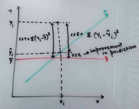
In this case, SSE is called Sum of Square Total, SST = Σ(Y(x) - Y̅)² (also called variance of Y)

The error SST is considered as a reference for Linear Regression Models to be evaluated as we start including independent variables. This is because, the error metric is supposed to decline with increase in variables (otherwise including the variable is useless).

Case 2:

After inclusion of independent variables, the error metric i.e. SSE = Σ(Y(x) - h_θ(x))² = Σ(Y(x) - Ŷ(x))²

Intutively, SST is the error of Y with no independent variable (Total variance) while SSE is the error of Y with independent variables included (Unexplained variance). From this, we can compute the variance that model in case 2 is able to explain compared to case 1. Let’s call it SSR (Sum of Square of Regression also called explained variance).

So, SSR = SST - SSE

Now we can define another evaluation metric for our model i.e. R-Squared = (Explained Variance)/(Total Variance)

R² = SSR/SST = (SST - SSE)/SST = 1 - (SSE/SST)

R² varies between 0 and 1. Higher the R² ⇒ better the model. (Caution! Overfitting)

Mathematically, R² may have negative values. However, when this happens, the error of the model is greater than SST, so the predicitons are worse than the average predictions with no independent variables and model is useless. This situation might arise in certain cases of overfitting when validating model with test data.

Overfitting

Once the model is built on the data (called as train data), we have to test it against unseen or out of sample data (called as test data) to verify that the patterns or equations discovered apply to them as well. Often, it so happens that while trying to learn the relationship, we end up learning the noise present in the data as well. This leads to really good results for the train data but when applied to test data, the result declines.

In order to prevent overfitting, instead of relying on R² alone (R² will always increase as we increase no. of variables), a new metric is designed, Adjusted R-Squared.

Adj R² = 1 - ^{(1 - R2)*(n - 1)}⁄_{(n - p - 1)}, where, n is no. of data points and p is no. of variables.

From the equation above, as p increases (Keeping R² constant) ⇒ Adj R² decreases, but since we know that as p increases ⇒ R² increases, and from the equation again, as R² increases ⇒ Adj R² increases. So, it’s a battle between p and R² that will decide if Adj R² will increase or decrease. If increase in p does not increase R² to a certain limit, Adj R² decreases. Hence, Adj R² is often used as the metric to come up with optimum list of variables in the final model.

Theory

• Normal Equation Method -

This method is based on Linear Algebra.

Y = Xβ + ε

Matrix Representation -

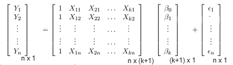
So, ε = Y - Xβ

Now, our error metric SSE can be represented in matrix form as, εʹε = ε₁² + ε₂² + … + ε_n² = Σε_i²

Therefore, εʹε = (Y - Xβ)ʹ(Y - Xβ)

⇒ εʹε = YʹY - YʹXβ - βʹXʹY + βʹXʹXβ

Here, 2nd and 3rd term on the RHS are transpose of each other. Also, they are scalar values with dimension (1 x 1). So, they are equal to each other.

⇒ εʹε = YʹY - 2βʹXʹY + βʹXʹXβ

Now, the above equation is a function of β and our objective is to minimize it. In order to do this, we differentiate the equation with respect to β and equate to Zero.

⇒ ^∂(εʹε)⁄_∂β = -2XʹY + 2XʹXβ = 0

⇒ XʹXβ = XʹY

Now, Pre multiplying by inverse of XʹX

⇒ (XʹX)^-1XʹXβ = (XʹX)^-1XʹY

⇒ Iβ = (XʹX)ʹXʹY ; where I is the identity matrix

⇒ β = (XʹX)^-1XʹY

If we analyze the above equation, the first term XʹX is the covariance matrix of independent variables while second term XʹY is covariance between X and Y. This can be easily seen when we consider the variables in their standardized form (Standard Normal Distribution).

• Gradient Descent -

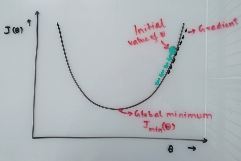
Gradient tells us the slope of a function at a given position. It is a vector which always points towards the maximum increase of a function. So, the general procedure is to define the objective function, randomly initialize parameters and gradually move in the opposite direction as that of the gradient in order to minimize the function’s value.

The Objective function we have is SSE. Let’s denote it by J(θ) = ¹⁄_2nΣ{h_θ(x⁽ⁱ⁾) - Y⁽ⁱ⁾}²; where i = 1 to n. n is no. of observations and k is no. of variables.

The function is same as the one considered before with slight additions. The additional term 1⁄2 is for mathematical convenience while n is merely to make the error metric MSE(Mean Square Error). This would not affect the output that we get.

Gradient of J is defined as, ^∂J(θ)⁄_∂θj = ¹⁄_nΣ{h_θ(x⁽ⁱ⁾) - Y⁽ⁱ⁾}x⁽ⁱ⁾_j; where j = 0 to k.

The update equation for θ,

Repeat untill Convergence, θ_j:= θ_j - α^∂J(θ)⁄_∂θj; where α is learning rate.

α is a hyperparameter that varies between 0 and 1 and needs to be optimized. After every update we calculate J(θ) and observe the change. This updation of θ might go on forever, so, we define a stopping criteria (often called precision) for when we are very close to the global minima of the function. If the change is less than the specified precision i.e. convergence is achieved, the algorithm stops.

Note: The update for all the θs happen simultaneously.

The process described above is called Batch Gradient Descent.

An alternate process is Stochastic Gradient Descent where we update θs based on 1 data point at a time. The data points are chosen randomly(stochastic). Another alternate approach is Mini Batch Gradient Descent where we update θs based on certain fixed no. of data points at a time.

Python Code

• Batch Gradient Descent

I will write a separate post explaining the Assumptions of Linear Regression and its usage on a dataset.