Logistic Regression

Logistic Regression is one of the most popular algorithms and is used widely in the industry. It is a classification model that gives out probability of occurence of an event. For eg, if you want to determine if a customer is going to default on his loan from a bank based on his historical behaviour, logistic regression is one of the models you would be using. Since, it is a classification technique, it is used for categorical target variables.

Theory

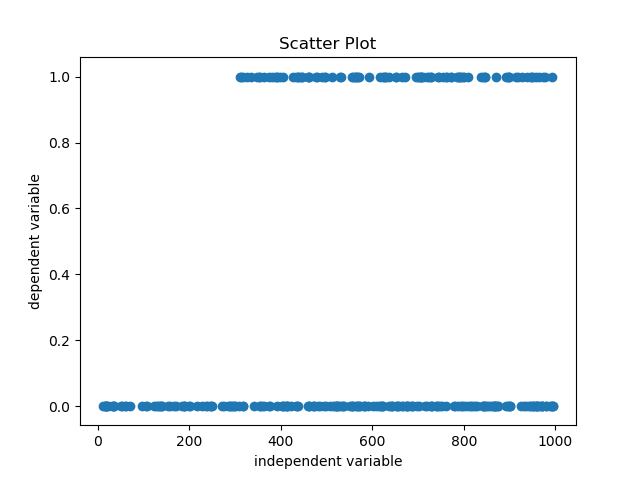
Below is a scatter plot for a continuous predictor and a categorical target variable-

From the plot it is very obvious that a linear equation like model (linear regression) would not work in it’s raw form as the output of linear regression would be unbounded and we would need some sort of transformation to bring the output in the permissible range of probability i.e. (0,1). In case of logistic regression, we use logit transformation for this purpose.

Z(x) = θ_o + θ₁x₁ + θ₂x₂ + … + θ_nx_n

Logit Transformation (also defined as log(odds)), Z(x) = ln(^P(x)⁄_1-P(x)); where ln is natural log.

⇒ P(x) = 1/(1+e^-Z(x));

where x₁, x₂, …. , x_n are independent variables, θ_o, θ₁, … , θ_n are coefficients of independent variables and P(x) is the probability of occurence of event.

which is also the General Equation of a logistic regression with n independent variables.

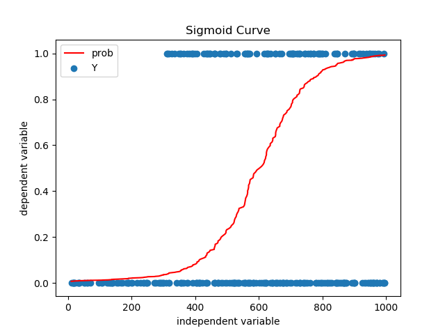
The red line in the plot above is the probability output. It looks like S-shaped curve and is also called Sigmoid Curve.

In order to use these probabilities for classification purpose, a threshold value is decided between 0 and 1, below which all the predictions will be decided as 1 and all the rest as 0. As a naive rule, 0.5 can be taken as the cutoff, but there are better methods to determine the same. We will discuss these later.

Probability (Revision)

In probability, it’s very important to define the sample space (Total possible outcomes, represented as S). The probability of occurence of an event E, is defined as, P(E) = Favourable Outcomes/ Total Possible Outcomes. So, P(E) = n(E)/n(S)

Eg - Event is Rolling a dice and getting a 4. There is total 6 faces on the dice with numbers 1 to 6 on it. So, favourable outcome is when we get 4 i.e. one case and total possible outcomes is six. ⇒ P(4 on dice) = 1/6.

Now, there are some terms that one should be aware of when discussing probability.

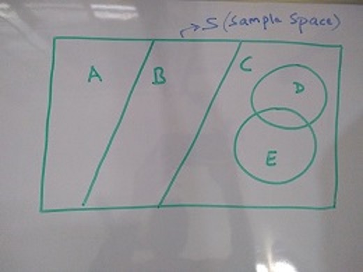
• Exhaustive Events - The set of events that forms the sample space i.e. no event can take place outside this set.

• Mutually Exclusive Events - Events that can not take place together. They are also called disjoint events.

  Sum of probabilites of events that are mutually exclusive and exhaustive is 1 i.e. Σ P(E_i) = 1 where i = 1,2,3,..,n(S)

In the above image, events D and E are subsets of event C. Event A, B and C together form set of exhaustive events and are mutually exclusive. Event D and E are not mutually exclusive as they have a non zero intersection part. So, P(A) + P(B) + P(C) = 1.

• Independent Events - If occurence or non occurence of an event A does not affect the occurence of another event B, then A and B are said to be independent events. In order to understand this better, we have to look for conditional probabillity.

P(A/B) => read as Probability of occurence of event A when it is known that Event B has already occured. (Probability of A given B)

Since, Event B has already occured, the set of possible outcomes has now reduced to n(B), So favourable outcomes for A are only going to be from the set n(B) ⇒ We have to look for the ones where A and B occurs simultaneously.

⇒ P(A/B) = n(A∩B)/n(B) = ^{n(A∩B)/n(S)}⁄_n(B)/n(S) = P(A∩B)/P(B)

⇒ P(A∩B) = P(A/B)*P(B)

Now, P(A) changed after occurence of B => it became P(A/B). What happens when P(A/B) = P(A)?

Intuitively, it means occurence of B did not affect A i.e. B has no effect on A ⇒ A and B are independent events.

⇒ P(A∩B) = P(A) * P(B) ⇒ Condition of Independence.

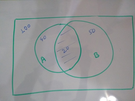
If we look at above image, we see that, P(A) = 40/100 = 0.4 (A occurs 40 out of 100 times). Now, When we try to calculate P(A/B), our sample space reduced to 50(no. of times B is occuring). Out of these 50, there are 20 times A can occur. So, P(A/B) = 20/50 = 0.4.

We can also look at it the other way, through the condition we derived.

P(A∩B) = 20/100 = 0.2

Also, P(A) * P(B) = 40/100 * 50/100 = 0.4*0.5 = 0.2

Hence, what we see above is an example of independent events. This condition of independence can be extended to n no. of events being independent of each other i.e.

⇒ P(A∩B∩C) = P(A) * P(B) * P(C) and so on.

• Odds = P(occurence)/P(non occurence) =p/(1-p)

Eg - For a fair coin toss, odds of getting a head = P(Head)/P(Not Head) = P(Head)/P(Tail) = 0.5/0.5 = 1:1

• Odds Ratio = Ratio of two odds = Odds1/Odds0

Eg - For a fair coin toss, P(Head) = 0.5 ⇒ Odds(Head) = Odds0 = 1:1

For an unfair coin, let’s say, P(Head) = 0.6 ⇒ Odds(Head) = Odds1 = 0.6:0.4 = 3:2

Therefore, Odds Ratio = Odds1/Odds0 = 1.5

This means, Odds of getting a head on the unfair coin is 1.5 times higher than the fair coin.

But, Why are we talking about Odds and Odds Ratio all of a sudden?

That’s because in the output of logistic regression, Odds Ratio of a variable can be defined as the increase in odds of Event happening with unit increase in corresponding variable and it remains constant irrespective of the value from which the unit increase has been made. Note: Probability might still be less with higher value for Odds Ratio.

Explanation :

log(odds0) = ln(^P(x)⁄_1-P(x)) = θ_o + θ₁x₁ + θ₂x₂ + … + θ_nx_n

⇒ odds0 = e^{θ_o + θ₁x₁ + θ₂x₂ + … + θ_nx_n}

Let’s increase the value of variable x₁ by 1 keeping other variables constant.

So, log(odds1) = θ_o + θ₁(x₁ + 1) + θ₂x₂ + … + θ_nx_n

⇒ odds1 = e^{θ_o + θ₁(x₁ + 1) + θ₂x₂ + … + θ_nx_n}

Therefore, odds ratio of x₁ = odds1/odds0 = e ^θ₁ which is constant for a given dataset. Also, Note that this is independent of the value of x₁ from which the increment was made.

Algorithm

In Logistic Regression, we use Maximum Likelihood Estimation in order to arrive at the coefficients of the variables.

• Maximum Likelihood Estimation -

The equation we have at hand is, P(x⁽ⁱ⁾) = h_θ(x⁽ⁱ⁾) = 1/(1+e^-Z(x(i))); where Z(x⁽ⁱ⁾) = θ^Tx⁽ⁱ⁾

Now, P(Y=1/x⁽ⁱ⁾;θ) = P(x)⁽ⁱ⁾ = h_θ(x⁽ⁱ⁾) (This means Y=1, x is known and θ is the unkown on which probability depends)

Also, P(Y=0/x⁽ⁱ⁾;θ) = 1 - P(x⁽ⁱ⁾) = 1 - h_θ(x⁽ⁱ⁾)

So, together, it can be represented as, P(Y⁽ⁱ⁾/x⁽ⁱ⁾;θ) = h_θ(x⁽ⁱ⁾)^Y(i) (1 - h_θ(x⁽ⁱ⁾))^(1-Y(i))

This equation is for a single data point. Now, in any linear model, it is one of the key assumption that the observations will be independent of each other i.e. occurence of event for one data point will not affect the occurence of event for another. Using this assumption, we can apply condition of independence and obtain the Joint Probability here,

P(Y/x;θ) = P(Y⁽¹⁾/x⁽¹⁾;θ) * P(Y⁽²⁾/x⁽²⁾;θ) * P(Y⁽³⁾/x⁽³⁾;θ) * …. * P(Y^(m)/x^(m);θ) ; where m is no. of data points.

⇒ P(Y/x;θ) = Π P(Y⁽ⁱ⁾/x⁽ⁱ⁾;θ) where i = 1,2,3,…,m

⇒ L(θ) = Π h_θ(x⁽ⁱ⁾)^Y(i) (1 - h_θ(x⁽ⁱ⁾))^(1-Y(i)) where i = 1,2,3,…,m and L(θ) is called Likelihood function.

This is our objective function and we are going to try and maximize it. For this we will be using Gradient Ascent(opposite of Gradient Descent) but first we need it in correct form to make calculations easy.

So, taking Log on both sides, we get log likelihood which is what we will be maximizing.

l(θ) = log(L(θ)) = Σ Y⁽ⁱ⁾ * log(h_θ(x⁽ⁱ⁾)) + (1 - Y⁽ⁱ⁾) * log(1 -h_θ(x⁽ⁱ⁾))

Gradient of l is defined as, ^∂l(θ)⁄_∂θj = Σ{Y⁽ⁱ⁾ - h_θ(x⁽ⁱ⁾)}x⁽ⁱ⁾_j; where j = 0 to n.

The update equation for θ,

Repeat untill Convergence, θ_j:= θ_j + α^∂l(θ)⁄_∂θj; where α is learning rate.

α is a hyperparameter that varies between 0 and 1 and needs to be optimized. It decides how fast or slow our algorithm is going to converge. Higher values might lead to overshooting the maxima and non convergence, while with lower values, it will take longer time to converge. After every update we calculate l(θ) and observe the change. This updation of θ might go on forever, so, we define a stopping criteria (often called precision) for when we are very close to the global maxima of the function. If the change is less than the specified precision i.e. convergence is achieved, the algorithm stops.

I will write a separate post explaining the implementation of Logistic Regression on a dataset. For understanding how we would evaluate the model built, refer to the below links -

Evaluation of Classification Algorithms-Part1

Evaluation of Classification Algorithms-Part2