Support Vector Machine

In this post, we will be looking at the classification technique known as Support Vector Machine (SVM). SVM is one of the most effective classification algorithms and is often found difficult to understand primarily because there are various kinds of concepts that are involved at play.

So far the algorithms that we have looked at (Linear and Logistic Regression) rely on Gradient Descent to achieve optimal values. However, SVM is slightly different. We will be using gradient here as well but not exactly in the same manner.

Introduction

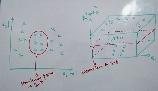
SVM gives us an option to transform the data into a higher dimension. It runs on an idea that if data is not linearly separable, we move to a higher dimension to find a plane that can separate the data linearly. In lower dimension, this might appear to be a non-linear plane. The reason it is called support vector machine is because the identified separator plane uses the nearest data points of each class to classify and these data points are called support vectors. This way, we are using the data point from class 1 that is most similar to class 2 and similarly the other way. The image below depicts this information.

SVM_support_vectors

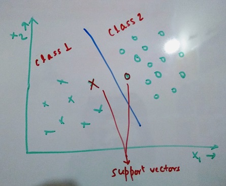
In the above image the points nearest to the plane are called support vectors. Below is an example of how changing the data to higher dimension helps separate the classes.

SVM_higher_dimension

Pre-Requisites

There are certain prerequisites that one should know before understanding how SVMs work. Let’s look at them -

Vectors and Planes -

Equation of a plane P : ax + by + cz = k (3-dimensional)
Normal Vector to the plane P (Vector perpendicular to the plane) : aî + bĵ + ck̂
Distance of a point Q(x₁,y₁,z₁) from the plane P : ± ^{(ax₁ + by₁ + cz₁ -k)} ⁄ _{√(a² + b² + c²)}

The distance would be represented with a modulus but the value itself would be (+) or (-) depending on which side of the plane the point lies.

Gradient - Gradient of a function is a vector that points towards the maximum increase of the function
General Fact - min_x max_α f(x,α) ≥ max_α min_x f(x,α)
Lagrangian Method - This method is used to find optimal values of a function subject to certain constraints.

Initial Form

Objective function : min_x f(x)

Equality Constraint : h(x) = 0

In order to solve this, we need to understand that the minima of f(x) will occur when both f(x) and h(x) are tangential to each other. ⇒ ∇_x f = -λ (∇_x h) (λ can be positive or negative)

therefore, in order to solve this problem, we define a new Lagrangian function, ℒ(x,λ) = f(x) + λ(h(x))

Now, our objective is to just minimize this function. The conditions for this would be -

∇_x ℒ = 0 and ∇_λ ℒ = 0

⇒ ∇_x f = 0 and h(x) = 0 (This was our original condition as well).

The λ here is called lagrangian multiplier and represents ^{∇ ℒ} ⁄ _{∇ h} (The rate of increase of ℒ as we relax the conditions on h)

Ext1 : It has been shown that this can be extended for multiple constraints as well which is shown below -

Objective function : min_x f(x)

Equality Constraint : h_i(x) = 0 where i = {1,2,3,…,n}

In this case, the Lagrangian function would be : ℒ(x,λ₁,λ₂,…,λ_n) = f(x) + Σλ_i h_i(x)

Ext2 : Another extension of this is when we introduce inequality constraint instead of equality constraint into the picture.

Objective function : min_x f(x)

Inequality Constraint : g(x) ≤ 0

New Lagrangian function - ℒ(x,α) = f(x) + α(g(x))

Here, if the x at which f(x) achieves minima satisfies the condition g(x) < 0 ⇒ the constraint is not required and α can be set to 0. If not, then again the minima will occur where both the functions are tangential to each other and so, g(x) = 0 (because the intersection point will lie on g(x))

⇒ α(g(x)) = 0 always and hence the function’s value at minima is again same as minima of f(x). α here is called KKT multiplier (KKT stands for Karush-Kuhn-Tucker)

Ext3 : Generalizing with both equality and inequality constraints -

Objective function : min_x f(x)

Equality Constraint : h_i(x) = 0 where i = {1,2,3,…,n}

Inequality Constraint : g_j(x) = 0 where j = {1,2,3,…,m}

The Lagrangian function in this case would be, ℒ(x,λ₁,λ₂,…,λ_n,α₁,α₂,…,α_m) = f(x) + Σλ_i h_i(x) + Σα_j g_j(x)

Primal and Dual Form - These are two forms of objective function and we are going to look at them using the generalized form mentioned above in Ext3.

Primal Form -

ℒ(x,λ₁,λ₂,…,λ_n,α₁,α₂,…,α_m) = f(x) + Σλ_i h_i(x) + Σα_j g_j(x) subject to the corresponding equality and inequality conditions.

The primal form is : θ_p(x) = max_α,λ ℒ(x,λ,α)

If the x satisfies the constraints, then θ_p(x) = f(x) as all the other terms are 0. So, our problem becomes, min_x θ_p(x) = min f(x) = p

Dual Form -

ℒ(x,λ₁,λ₂,…,λ_n,α₁,α₂,…,α_m) = f(x) + Σλ_i h_i(x) + Σα_j g_j(x) subject to the corresponding equality and inequality conditions.

The Dual form is : θ_d(α,λ) = min_x ℒ(x,λ,α)

So, entire problem, max_α,λ min_x ℒ(x,λ,α) = d

From the general fact mentioned above, min_x max_α f(x,α) ≥ max_α min_x f(x,α)

Comparing this with our situation, d ≤ p

The two values d and p are equal when they staisfy a set of condition called KKT conditions. Following are the condition,

i. ∇_x ℒ = 0

ii. ∇_λ ℒ = 0

iii. α_j ≥ 0

iv. g_j ≤ 0

v. α_j g_j = 0

All these conditions are satisfied in our case and hence, we can solve the dual form instead of primal form if the primal form turns out to be a non convex problem and cannot be solved.

Notation

The Notations used for SVM is slightly different from that of logistic regression where we used 0 and 1 for representing success and failure. SVM uses {-1, +1} for differentiating between classes. This technique uses vector approach and identifies a plane that separates both classes from each other.

Theory (Problem Formulation)

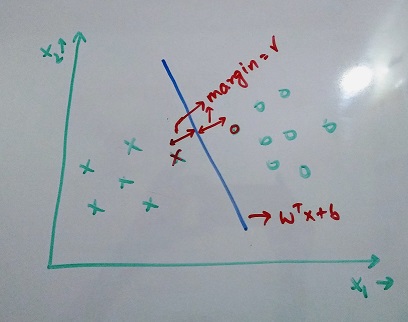
First we look at how SVM uses the data in it’s current form to identify the separation plane and then see how we can use it to transform the data into higher dimension. Since, we are using a plane to separate the classes. The objective function will be the equation of a plane.

h(w,b) = w^Tx + b (This is the equation of a plane in linear algebra form and is equivalent to ax + by + cz + k = 0 in 3-D)

where w = [θ₁,θ₂,…,θ_n], x = [x₁,x₂,…,x_n] and b = θ₀ in n-Dimnesion.

The objective is to maximize the distance between the nearest data point of each class (support vectors) and the plane. Below is an image showing a linearly separable dataset.

SVM_Margin

Also, y⁽ⁱ⁾(w^Tx⁽ⁱ⁾ + b) > 0 ⇒ data point correctly classified (If data point is on left side of the plane, the distance will be negative and if on the right side, it will be positive. This coupled with the notation of {-1, +1} always results in positive number for correct classifications)

Note: the denominator of distance has been omitted here as it is always positive (equivalent to √(a² + b² + c²))

This metric is called functional margin, γ̂ ⁽ⁱ⁾ = y⁽ⁱ⁾(w^Tx⁽ⁱ⁾ + b)

There is another metric called geometric margin, γ⁽ⁱ⁾ = ^{γ̂ ⁽ⁱ⁾} ⁄ _||w||

Let’s denote γ = min γ⁽ⁱ⁾

Defining Objective

So, our objective function would be, max _{γ, w,b} γ subject to constraint ^{y⁽ⁱ⁾(w^Tx⁽ⁱ⁾ + b)} ⁄ _||w|| ≥ γ

This basically means, we want to maximize the minimum margin with constraint that the distance between every data point and the plane is greater than or equal to this value. Representing this in the form of functional margin,

max _{γ, w,b} ^γ̂ ⁄ _||w|| subject to constraint y⁽ⁱ⁾(w^Tx⁽ⁱ⁾ + b) ≥ γ̂

This problem is not solvable in its current form and hence, we need to perform certain manipulations. Notice in the definition of functional margin, γ̂ ⁽ⁱ⁾ = y⁽ⁱ⁾(w^Tx⁽ⁱ⁾ + b), if we change w → 2w and b → 2b ⇒ γ̂ → 2γ̂

This shows that it’s possible to choose a proportional value and rescale the entire objective to have maximum functional margin = 1. Therefore, on rescaling we get our objective function as,

max _{γ, w,b} ¹ ⁄ _||w|| subject to constraint y⁽ⁱ⁾(w^Tx⁽ⁱ⁾ + b) ≥ 1

This will be same as, min _{γ, w,b} ^||w||² ⁄ ₂ subject to constraint y⁽ⁱ⁾(w^Tx⁽ⁱ⁾ + b) ≥ 1

Theory (Problem Solution)

Lagrangian Method

In order to solve our problem, we will be using the Lagrangian Method described above in the pre-requiste section. Here, we have an objective function we want to minimize subject to an inequality constraint.

So, objective function : f(w) = ^||w||² ⁄ ₂

Inequality constraints : g_i(w,b) = - y⁽ⁱ⁾(w^Tx⁽ⁱ⁾ + b) + 1

Therefore, we define a lagrangian function, ℒ(w,b,α) = ^||w||² ⁄ ₂ - Σ_i^m α_i [y⁽ⁱ⁾(w^Tx⁽ⁱ⁾ + b) - 1]

Conditions to minimize the lagrangian is, ∇_w L = 0 and ∇_b L = 0

Applying these conditions, we get, w = Σ_i=1^m α_i y⁽ⁱ⁾ x⁽ⁱ⁾ and Σ_i=1^m α_i y⁽ⁱ⁾ = 0 - (Reference Equation 1)

Once, we get w (the value that decide the orientation of the plane), to obtain b (decides the parallel movement of plane) is easy. The plane would be at the mid point of the distance between closest data points of both classes (No class gets priority).

So, b = ^{max_{y = -1} w^Tx⁽ⁱ⁾ + min_{y = 1} w^Tx⁽ⁱ⁾} ⁄ ₂

Also, replacing the value of w in our prediction function, w^Tx + b = (Σ_i=1^m α_i y⁽ⁱ⁾ x⁽ⁱ⁾)x + b

⇒ w^Tx + b = Σ_i=1^m α_i y⁽ⁱ⁾ (x⁽ⁱ⁾)^Tx + b

Observe the term, (x⁽ⁱ⁾)^Tx. This is the product of training data points and new data point to be classified. It is also written as <x⁽ⁱ⁾,x> and is also called inner product.

If we look carefully at the prediction function, the value of α_i = 0 whenever g_i(w,b) ≠ 0 (Refer Prerequisite above) and hence, the prediciton will only depend on those training data points where g_i(w,b) = 0. This happens only for the data points closest to the plane. This is the reason these closest data points are called support vectors.

Now, the only thing unknown to us is α_i. For this, we will be using the primal and dual form explained above in the pre-requisite section.

Primal and Dual Form

Primal Form of the Lagrangian function, θ_p = max_α ℒ(w,b,α) = f(w,b)

So the objective becomes : min_w,b f(w,b) (This is again not solvable. Hence, we resort to Dual form of the problem)

and Dual Form of the Lagrangian function, θ_d = min_w,b ℒ(w,b,α)

Let’s solve the Lagrangian first by using value of w obtained above in order to calculate θ_d

ℒ(w,b,α) = ^||w||² ⁄ ₂ - Σ_i=1^m α_i [y⁽ⁱ⁾(w^Tx⁽ⁱ⁾ + b) - 1]

⇒ ℒ(w,b,α) = ^{(Σ_i=1^m α_i y⁽ⁱ⁾ x⁽ⁱ⁾)(Σ_j=1^m α_j y^(j) x^(j))} ⁄ ₂ - Σ_i^m α_i [y⁽ⁱ⁾ { (Σ_j=1^m α_j y^(j) x^(j)) x⁽ⁱ⁾ + b} - 1]

⇒ ℒ(w,b,α) = ^{(Σ_i,j=1^m α_iα_j y⁽ⁱ⁾y^(j) (x⁽ⁱ⁾)^T x^(j))} ⁄ ₂ - Σ_i,j=1^m α_iα_j y⁽ⁱ⁾y^(j) (x⁽ⁱ⁾)^T x^(j) - b Σ_i=1^m α_i y⁽ⁱ⁾ + Σ_i=1^m α_i

From Reference Equation 1 above, the third term is 0

⇒ ℒ(w,b,α) = Σ_i=1^m α_i - (¹⁄₂)Σ_i,j=1^m α_iα_j y⁽ⁱ⁾y^(j) (x⁽ⁱ⁾)^T x^(j)

Now, the above equation is only a function of α_i. So pluging this into our dual form,

max_α θ_d(α) = max_α Σ_i=1^m α_i - (¹⁄₂)Σ_i,j=1^m α_iα_j y⁽ⁱ⁾y^(j) (x⁽ⁱ⁾)^T x^(j) subject to contraints α_i ≥ 0 and Σ_i=1^m α_i y⁽ⁱ⁾ = 0

⇒ max_α θ_d(α) = max_α Σ_i=1^m α_i - (¹⁄₂)Σ_i,j=1^m α_iα_j y⁽ⁱ⁾y^(j) <x⁽ⁱ⁾,x^(j)> subject to contraints α_i ≥ 0 and Σ_i=1^m α_i y⁽ⁱ⁾ = 0

SMO Algorithm

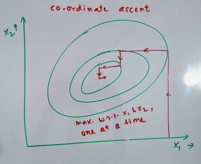
The way we solve this is, we vary two α’s at a time and optimize the function according to it (We cannot vary one at a time because varying one keeping others constant would violate the second constraint). So, vary α₁ and α₂ together.

α₁y₁ + α₂y₂ = k

⇒ α₁ = ^{(k - α₂y₂)} ⁄ _y₁

therefore, θ_d(α) will be of the form aα₂² + bα₂ + c which is a solvable quadratic equation. Post this, we will maximize the function for another set of α’s. This is called as Sequential Minimal Optimization (SMO Algorithm). Following image describes how this would work when varying one α at a time in 2-D (Coordinate Ascent Algorithm)

Coordinate_ascent

Kernels

A very important point to notice above is in both the prediction function and the final objective function, the involvement of data point is in their inner product form <x⁽ⁱ⁾,x^(j)>. The values x⁽ⁱ⁾ and x^(j) here are the feature sets of data and this form helps us as we can just replace them with any other feature set and nothing else needs to change. The other feature set is generally one with a higher dimension and is represented in inner product form as <Φ(x)⁽ⁱ⁾,Φ(x)^(j)>.

This higher dimension can be computationally very inefficient and might take very long time to calculate but what if we could somehow represent this inner product through some function that can be computed very easily. These functions are called Kernal function. Let’s take an example for this -

Let K(x,z) = (x^Tz)²

⇒ K(x,z) = (Σ_i=1^m x_iz_i) (Σ_j=1^m x_jz_j)

⇒ K(x,z) = Σ_i,j=1^m (x_ix_j)(z_iz_j)

So, if we consider x to be in 3-D, here Φ(x) = [x₁x₁, x₁x₂, x₁x₃, x₂x₂, x₂x₃, x₃x₃]

By considering the Kernel function mentioned above, we moved from 3-D to 6-D space. Also, this way instead of calculating the Φ(x), we directly calculate the inner product which is computationally very efficient.

There are lots of commonly used Kernel functions with the most common being Guassian Kernel, K(x,y) = exp(- ^{||x - y||²} ⁄ _2σ²)

In order to see the φ(x) for guassian kernel, we can use taylor expnasion for exp(x). This will show us that this kernel takes our data to infinite dimensional space.

End Notes

I would recommend going through the derivations by writing them yourself as that would clear up a lot of concepts. Let me know if any clarifications are needed in the comments section below.

I would be adding implementation of SVM on a dataset shortly.