Assumptions of Linear Regression

In the last post, I described the workings of a Linear Regression Model. Now, with any model there is a randomness (error or residual) associated which we call the noise in the data. Usually, we can represent it as Data = Formula + Noise. For us to understand how good our model is, we should explore this randomness for any improvements possible.

General equation for linear regression with n independent variables is,

Y(x) = θ_o + θ₁x₁ + θ₂x₂ + … + θ_nx_n + ε

Following are the assumptions that we should be checking in case of a Linear Regression Model:

• Linearity - The independent variables should be having a linear relationship with the dependent variable. This is inherently because we are trying to build a linear model and any non linearity would not be taken into account by our linear equation. The implications can be severe deflections of predictions from actual values. This happens when model is used to extrapolate beyond range of data on which model was built on. This assumption can be verified by simply looking at the scatter plot between the variables.

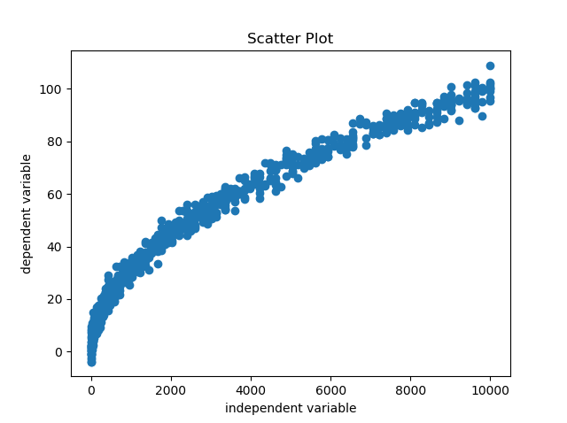
In case we find any non linear relationship appearing in the scatter plot like the one above, it should be used to apply transformations on the independent variable. Here, since the relationship appears quadratic, we will apply square root on the independent variable and check the scatter plot once again.

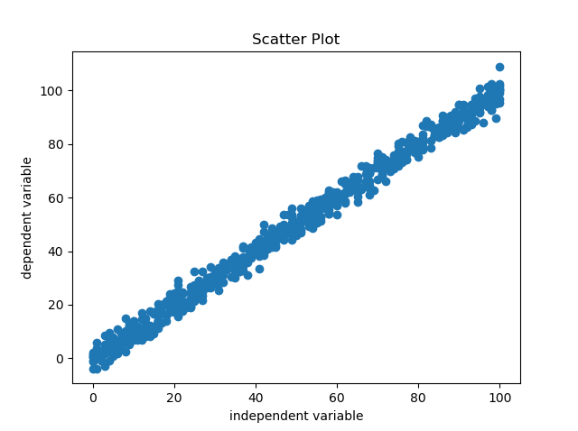
Since, now the relationship is linear, we are good to include the variable in the model.

• Normality of Residuals - The residuals of a linear regression model are supposed to follow normal distribution mainly because of two reasons. One being mathematical convenience and other being Central Limit Theorem. This assumption can be checked via histogram of residuals.

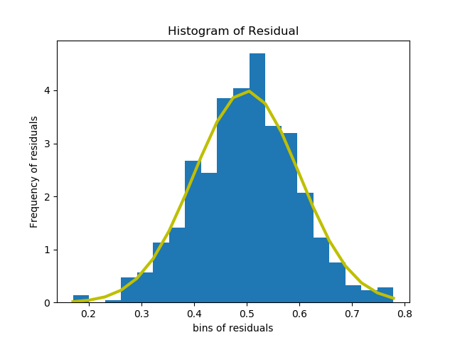
In case we don’t get a normal distribution out of the histogram, it means the confidence intervals we get from the model would not be much reliable but the model can still be considered for predictions. So, this assumption is not very important if one is only interested in predictions.

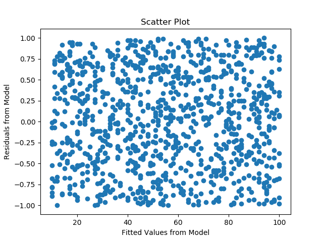
• Constant Error Variance of Residuals (Homoscedasticity) - The Residuals are also expected to be uniformly distributed across the data. This assumption I feel somehow ties back to the first assumption of linearity. If the variance in error is not constant throughout the range of data, it means we are missing a factor in our model that will help us obtain better results. This can be checked by plotting residuals against the fitted values or residuals against time for a time series data.

Below is the graph of a Homoscedasticity.

Below is an example of error variance not being constant i.e. heteroscedasticity.

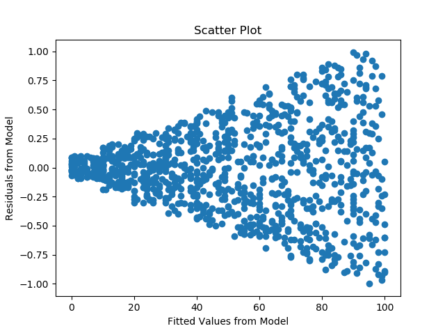
The variance of error not being constant means there is a scope of improvement in the model and we are missing out on an important factor.

• Independence of Residuals - One of the basic assumption of any linear model is that the observations are not correlated with each other. This means that presence of high value in the data should not mean the subsequent value is also going to be high or vice versa. If this happens, then we are most probably dealing with time series data and there are other models that we should be using instead.

This can be checked by evaluating autocorrelation for the dependent variable or plotting residuals of the model in the order they appear in the data. For the assumption to be verified, the plot should be random and no pattern should be visible.

In the plot above, there is a clear pattern emerging from the plot of residuals which means that the errors are not independent of each other and the occurence of a data point is affected by the subsequent ones. In this case, we should use a time series model instead.

Apart from these assumptions we should also check for presence of multicollinearity in the data.

Multicollinearity

This refers to the situation where the independent variables (predictors) are highly correlated among each other. The problem with this is, if we look at the equation of linear regression, we say a unit change in x₁ results in θ₁ amount of change in Y, given other predictor variables are constant but, in presence of high correlation, there’s a good chance (correlation vs causation) other variables won’t remain constant.

This can be checked by looking at the correlation matrix for the predictors. Another way of determining this would be to consider Variance Inflation Factor(VIF). VIF is calculated for each and every predictor without taking the outcome variable into consideration.

Calculation of VIF :

Suppose we have 4 independent variables x₁, x₂, x₃ & x₄ and Y is the dependent variable. For obtaining VIF for x₁, a linear regression model is built with x₁ as outcome and x₂, x₃ & x₄ as predictors. Next, we look at the R Squared for this model. This will tell us if x₁ can be predicted by using other independent variables. This process is repeated for every predictor variable.

VIF = 1/(1-R²)

So, a R² of 0.9 would be equivalent to VIF of 10. The general thought is that, if a variable can be predicted using other predictor variables, then it is replacable in the linear regression equation.

Y(x) = θ_o + θ₁x₁ + θ₂x₂ + … + θ_nx_n + ε

and, x₁ = θ_ox1 + θ_2x1x₂ + … + θ_nx1x_n + ε_x1

Replacing x₁ in Y, Y(x) = θ_o + θ₁(θ_ox1 + θ_2x1x₂ + … + θ_nx1x_n + ε_x1) + θ₂x₂ + … + θ_nx_n + ε

Once we have VIF calculated for all the predictors, a threshold is decided beyond which we will start dropping variables from the model. This a recursive process where the variable with highest VIF is dropped one at a time. After dropping a variable, VIF is recalculated and the process is repeated until all the variables are within the decided VIF threshold. Generally, a threshold of 4 is considered for VIF but this can vary based on business requirements and problem statement.

Link to usage of Linear regression on a dataset - Here